Scientific Programming with Python¶

Outline¶

Introduction to Python
Python for science, where to begin?
Python language
Scientific libraries

Introduction to Python¶

What is Python?¶

Python is a modern, general-purpose, object-oriented, high-level programming language.

General characteristics of Python:

clean and simple language: Easy-to-read and intuitive code, easy-to-learn minimalistic syntax, maintainability scales well with size of projects.
expressive language: Fewer lines of code, fewer bugs, easier to maintain.

Advantages:¶

The main advantage is ease of programming, minimizing the time required to develop, debug and maintain the code.
Well designed language that encourage many good programming practices:
- Modular and object-oriented programming, good system for packaging and re-use of code. This often results in more transparent, maintainable and bug-free code.
- Documentation tightly integrated with the code.
A large standard library, and a large collection of add-on packages.
Packaging of programs into standard executables, that work on computers without Python installed.

Disadvantages:¶

Since Python is an interpreted and dynamically typed programming language, the execution of python code can be slow compared to compiled statically typed programming languages, such as C and Fortran.
Somewhat decentralized, with different environment, packages and documentation spread out at different places. Can make it harder to get started.

Python has a strong position in scientific computing
- Large community of users, easy to find help and documentation.
Extensive ecosystem of scientific libraries
- NumPy: numerical Python $\approx$ MATLAB matrices and arrays
- SciPy: scientific Python $\approx$ MATLAB toolboxes
- pandas: extends NumPy
- Matplotlib: graphics library
- Sympy: symbolic mathematics library
Scientific (and non-scientific) development environments available
- spyder: MATLAB-like environment
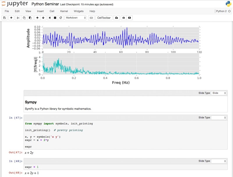
- Jupyter/IPython notebooks: environment for interactive and exploratory Python
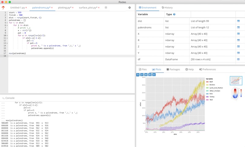
- Rodeo: new Python environment for data science
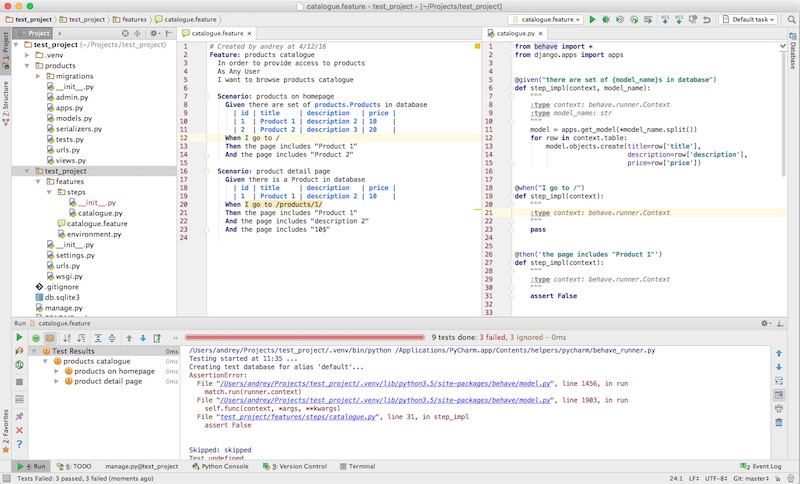
- PyCharm: Python enviroment for developers
Great performance due to close integration with time-tested and highly optimized codes written in C and Fortran
Readily available and suitable for use on high-performance computing clusters
No license costs, no unnecessary use of research budget

Python for science, where to begin?¶

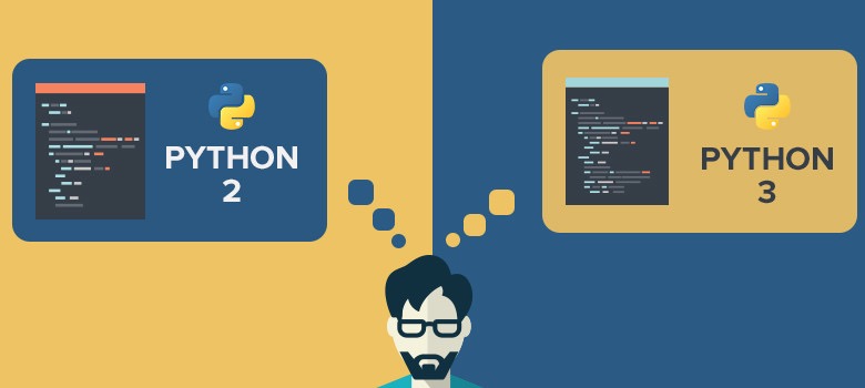
Why to choose Python 2?¶

Python 3 is better, but some non-widespread science modules are still not compatible
Differences between Python 2 and 3 are relatively minor
Python 2 is actively supported. For example, Linux distributions and Macs are still using 2.x as default

Scientific-oriented Python Distributions¶

Provide a Python interpreter with commonly used scientific libraries in science like NumPy, SciPy, Pandas, matplotlib, etc. already installed. In the past, it was usually painful to build some of these packages. Also, include development environments with advanced editing, debugging and introspection features.

Anaconda
- Cross-platform
- Supports Python 2 and 3
- Most widely adopted
Canopy
- Cross-platform
- Only supports Python 2
Python(x,y)
- Windows-only platform
- Only support Python 2

Anaconda navigator¶

Anaconda navigator: installing new packages¶

spyder¶

IPython/Jupyter notebooks¶

Rodeo (need to be installed separately from Anaconda)¶

PyCharm (need to be installed separately from Anaconda)¶

Editor	Learning curve	Users	Benefits
spyder	pretty short	Matlab and R background	mature, many features
rodeo	pretty short	Matlab and R background	modern, essential features
IPython/Jupyter	smooth	teachers	interactive
PyCharm	moderate	developers	code quality

Where to look for help?¶

Official documentation: http://www.scipy.org/docs.html
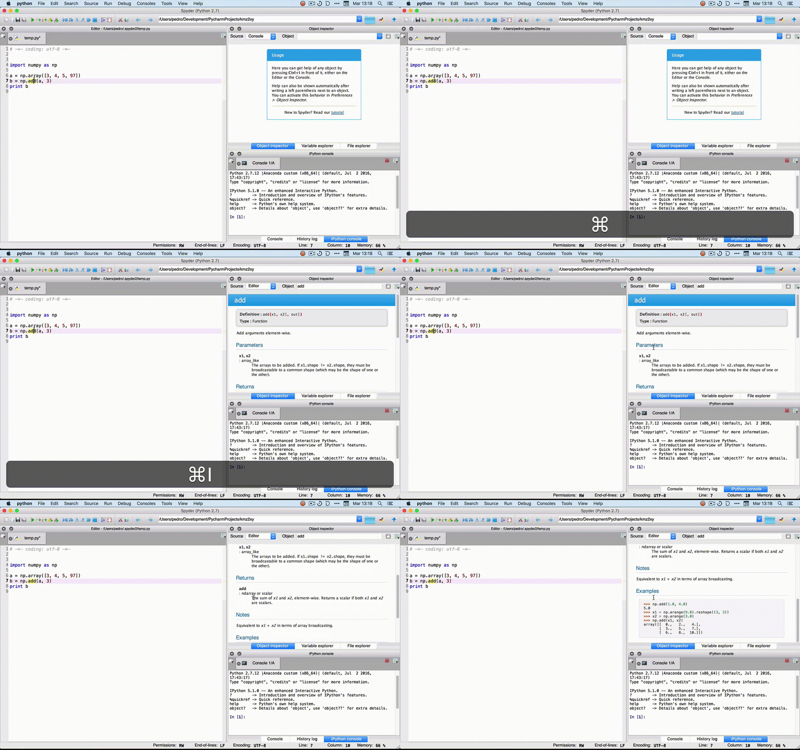
Usually included in development environments as contextual help:
- spyder: Ctrl+I (Windows) or Cmd+I (Mac)
- PyCharm: F1 (Windows/Mac)
- Rodeo: ?f in the console
Be careful about code you get on the internet!

Python language¶

Using Python as a Calculator¶

In [1]:

2 + 2

Out[1]:

In [2]:

17 / 3  # int / int -> int

Out[2]:

In [3]:

from __future__ import division
17 / 3

Out[3]:

5.666666666666667

Strings¶

In [4]:

prefix = 'Py'
word = prefix + 'thon'

# character in position 0
print word[0]

# characters from position 0 (included) to 6 (excluded)
print word[0:6]

P
Python

Note¶

0-based indexing

half-open range indexing: [a, b)

print statement to get outputs

line comments

Lists¶

In [5]:

# empty list
squares = []

# lists might contain items of different types
squares = ['cat', 4, 3.2]

# negative indices mean count backwards from end of sequence
print squares[-1]

# list concatenation
squares = squares + [81, 'dog']

# list functions
squares.remove(3.2)  # remove the first ocurrence
squares.append('horse')  # concatenation: same as +

print squares

3.2
['cat', 4, 81, 'dog', 'horse']

In [6]:

a = ['a', 'b', 'c']
n = [1, 2, 3]

# it is possible to nest lists
# (create lists containing other lists)
x = [a, n]

print x
print x[0]
print x[0][1]

[['a', 'b', 'c'], [1, 2, 3]]
['a', 'b', 'c']
b

Simple code: Fibonacci series¶

In [7]:

a, b = 0, 1
while a < 10:
    print a,
    # the sum of two elements defines the next
    a, b = b, a + b

0 1 1 2 3 5 8

Note¶

indentation level of statements is significant

multiple assignment

`if` Statements¶

In [8]:

x = -4

if x < 0:
    x = 0
    print 'Negative changed to zero'
elif x == 0:
    print 'Zero'
elif x == 1:
    print 'Single'
else:
    print 'More'

Negative changed to zero

`for` Statements¶

In [9]:

words = ['cat', 'window', 'defenestrate']

for w in words:
    # len returns the number of items of an object.
    print w, len(w)

cat 3
window 6
defenestrate 12

Warning¶

Please avoid Matlab-like for statements

In [10]:

for w in range(len(words)):
    print words[w], len(words[w])

cat 3
window 6
defenestrate 12

range(stop)

Built-in function to create lists containing arithmetic progressions.

In [11]:

print range(10)
print range(0, 10, 3)
print range(0, -10, -1)

[0, 1, 2, 3, 4, 5, 6, 7, 8, 9]
[0, 3, 6, 9]
[0, -1, -2, -3, -4, -5, -6, -7, -8, -9]

In [12]:

for i in range(4):
    print 'cat',

cat cat cat cat

In [13]:

words = ['cat', 'window', 'defenestrate']

for i, w in enumerate(words):
    print i, w

0 cat
1 window
2 defenestrate

Functions¶

In [14]:

def fib(n):
    """Build a Fibonacci series up to n.

    Args:
        n: upper limit.

    Returns:
        A list with a Fibonacci series up to n.
    """
    f = []  # always initialize the returned value!

    a, b = 0, 1
    while a < n:
        f.append(a)
        # the sum of two elements defines the next
        a, b = b, a + b

    return f

# now call the function we just defined:
print fib(1000)

[0, 1, 1, 2, 3, 5, 8, 13, 21, 34, 55, 89, 144, 233, 377, 610, 987]

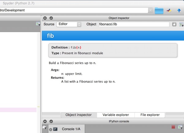
Functions: documentation strings (docstrings)¶

Python documentation strings (docstrings) provide a convenient way of associating documentation with Python functions and modules.
Docstrings can be written following several styles. We use Google Python Style Guide.
An object's docsting is defined by including a string constant as the first statement in the function's definition.
Unlike conventional source code comments the docstring should describe what the function does, not how.
All functions should have a docstring.
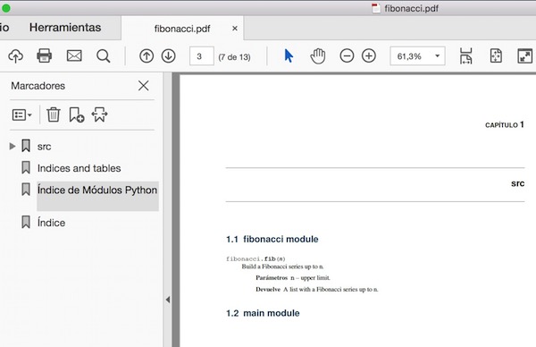
This allows to inspect these comments at run time, for instance as an interactive help system, or export them as HTML, LaTeX, PDF or other formats.

Functions: default argument values¶

In [15]:

def fib(n, s=0):
    """Build a Fibonacci series up to n.

    Args:
        n: upper limit.
        s: lower limit. Default 0.

    Returns:
        A list with a Fibonacci series up to n.
    """
    f = []  # always initialize the returned value!

    a, b = 0, 1
    while a < n:
        if a >= s:  # lower limit
            f.append(a)
        # the sum of two elements defines the next
        a, b = b, a + b

    return f

print fib(1000, 15)
print fib(1000, 0)
print fib(1000)

[21, 34, 55, 89, 144, 233, 377, 610, 987]
[0, 1, 1, 2, 3, 5, 8, 13, 21, 34, 55, 89, 144, 233, 377, 610, 987]
[0, 1, 1, 2, 3, 5, 8, 13, 21, 34, 55, 89, 144, 233, 377, 610, 987]

Functions: keyword arguments¶

In [16]:

print fib(1000, 15)  # positional arguments
print fib(s=15, n=1000)  # keyword arguments

[21, 34, 55, 89, 144, 233, 377, 610, 987]
[21, 34, 55, 89, 144, 233, 377, 610, 987]

Functions: returning multiple values¶

In [17]:

def fib(n, s=0):
    """Build a Fibonacci series up to n.

    Args:
        n: upper limit.
        s: lower limit. Default 0.

    Returns:
        (f, l):

        * ``f``: list with a Fibonacci series up to n.
        * ``l``: length of Fibonacci series.
    """
    f = []  # always initialize return values!
    l = 0

    a, b = 0, 1
    while a < n:
        if a >= s:  # lower limit
            f.append(a)
        # the sum of two elements defines the next
        a, b = b, a + b
    l = len(f)  # number of elements

    return f, l

a, b = fib(1000)
print a
print b

c = fib(1000)
print c

[0, 1, 1, 2, 3, 5, 8, 13, 21, 34, 55, 89, 144, 233, 377, 610, 987]
17
([0, 1, 1, 2, 3, 5, 8, 13, 21, 34, 55, 89, 144, 233, 377, 610, 987], 17)

Functions: importing external functions¶

In [18]:

import fibonacci  # without .py extension

print fibonacci.fib(3)

[0, 1, 1, 2]

In [19]:

from fibonacci import fib

print fib(3)

[0, 1, 1, 2]

In [20]:

import fibonacci as f  # alias

print f.fib(3)

[0, 1, 1, 2]

Recommendation¶

The best way to import libraries is included in their official help

Some examples:

import math
import numpy as np
from scipy import linalg, optimize
import pandas as pd
import matplotlib as mpl
import matplotlib.pyplot as plt
import sympy

Code Style¶

Style Guide for Python Code: PEP8.
Use only English (ASCII) characters for variables, functions and files. It is possible to use non-English characters in strings and comments by adding the following line at the beginning of each file: # -*- coding: utf-8 -*-.
Name your variables, functions and files consistently: the convention is to use lower_case_with_underscores.
We all use single-quoted strings to be consistent. Nevertheless, single-quoted strings and double-quoted strings are the same. PEP does not make a recommendation for this, except for function documentation where tripe-quote strings should be used.

PEP8 exceptions:¶

Long lines¶

It is very conservative and requires limiting lines to 79 characters. We use all lines to a maximum of 119 characters. This is the default behaviour in PyCharm.

Disable checks in one line¶

Skip validation in one lines by adding following comment:

# nopep8

`datetime` data type¶

The datetime module supplies classes for manipulating dates and times. Avoid converting dates or times to int (datenum or similar).

In [22]:

from datetime import datetime, date, time
# Using datetime.combine()
d = date(2005, 7, 14)
t = time(12, 30)
dt1 = datetime.combine(d, t)

print dt1
print dt1.year

2005-07-14 12:30:00
2005

In [23]:

from datetime import timedelta

dt2 = dt1 + timedelta(hours=5)

print dt2

2005-07-14 17:30:00

timedelta([days[, seconds[, microseconds[, milliseconds[, minutes[, hours[, weeks]]]]]]])

All arguments are optional and default to 0. Arguments may be ints, longs, or floats, and may be positive or negative.

`boolean` data type¶

boolean values are the two constant objects False and True. In numeric contexts (for example when used as the argument to an arithmetic operator), they behave like the integers 0 and 1, respectively.

Nevertheless, other values can also be considered false or true:

the following values are considered false: 0, '', [], (), {}, None
all other values are considered true, so objects of many types are always true

Scientific libraries¶

NumPy¶

NumPy’s main object is the homogeneous multidimensional array (ndarray). It is a table of elements (usually numbers), all of the same type, indexed by a tuple of positive integers. In Numpy dimensions are called axes. The number of axes is rank.

In [31]:

import numpy as np

# defining arrays and matrices
Z = np.array([1, 3, 4])

A = np.array([[1, 1], 
              [0, 1]])
B = np.array([[2, 0],
              [3, 4]])

In [32]:

# selecting elements
print A[0, :]

# elementwise product with * operator!
print A * B

# matrix product
print np.dot(A, B)

[1 1]
[[2 0]
 [0 4]]
[[5 4]
 [3 4]]

In [33]:

from numpy.linalg import solve, inv  # linear algebra

a = np.linspace(-np.pi, np.pi, 10)
print a

a = np.array([[1, 2, 3], [3, 4, 6.7], [5, 9.0, 5]])
print a

b =  np.array([3, 2, 1])
print solve(a, b)  # solve the equation ax = b

[-3.14159265 -2.44346095 -1.74532925 -1.04719755 -0.34906585  0.34906585
  1.04719755  1.74532925  2.44346095  3.14159265]
[[ 1.   2.   3. ]
 [ 3.   4.   6.7]
 [ 5.   9.   5. ]]
[-4.83050847  2.13559322  1.18644068]

In [34]:

print inv(a)

[[-2.27683616  0.96045198  0.07909605]
 [ 1.04519774 -0.56497175  0.1299435 ]
 [ 0.39548023  0.05649718 -0.11299435]]

In [35]:

print a.transpose()

[[ 1.   3.   5. ]
 [ 2.   4.   9. ]
 [ 3.   6.7  5. ]]

ndim the number of axes (dimensions) of the array. In the Python world, the number of dimensions is referred to as rank.

shape the dimensions of the array. This is a tuple of integers indicating the size of the array in each dimension. For a matrix with n rows and m columns, shape will be (n, m). The length of the shape tuple is therefore the rank, or number of dimensions, ndim.

size the total number of elements of the array. This is equal to the product of the elements of shape.

dtype an object describing the type of the elements in the array. One can create or specify dtype’s using standard Python types. Additionally NumPy provides types of its own. numpy.int32, numpy.int16, and numpy.float64 are some examples.

Warning¶

When operating and manipulating arrays, their data is sometimes copied into a new array and sometimes not. For example, simple assignments make no copy of array objects or of their data.

Vectorization¶

Numpy arrays enable you to express batch operations on data without writing any for loops. This is usually called vectorization:

vectorized code is more concise and easier to read
fewer lines of code generally means fewer bugs
the code more closely resembles standard mathematical notation

But:

sometimes it's difficult to move away from the for-loop school of thought

Pandas¶

Pandas is a newer package built on top of NumPy and pandas objects are valid arguments to most NumPy functions:

fast and efficient Series (1-dimensional) and DataFrame (2-dimensional) heterogeneous objects for data manipulation with integrated indexing
tools for reading and writing data from different formats: CSV and text files, Microsoft Excel, SQL databases, HDF5...
intelligent label-based slicing
time series-functionality
integrated handling of missing data

In [37]:

import pandas as pd

# ignore the following commands
# just for the slides
pd.set_option("display.max_rows", 10)
pd.set_option("display.max_columns", 5)

simar = pd.read_table('WANA_2006008_Algeciras.txt', 
                      delim_whitespace=True, 
                      parse_dates= {'date' : [0,1,2,3]}, 
                      index_col='date', skiprows=70)

simar

Out[37]:

	Hm0	Tm02	...	VelV	DirV
date
1996-01-14 03:00:00	0.5	2.2	...	4.5	176.0
1996-01-14 06:00:00	0.5	2.3	...	4.3	193.0
1996-01-14 09:00:00	0.4	2.3	...	4.3	193.0
1996-01-14 12:00:00	0.7	2.6	...	8.7	118.0
1996-01-14 15:00:00	0.9	3.0	...	8.7	118.0
...	...	...	...	...	...
1996-12-31 09:00:00	2.5	4.4	...	17.1	241.0
1996-12-31 12:00:00	2.0	4.1	...	15.4	263.0
1996-12-31 15:00:00	2.0	4.1	...	15.4	263.0
1996-12-31 18:00:00	1.4	3.6	...	12.4	263.0
1996-12-31 21:00:00	1.4	3.5	...	12.4	263.0

2823 rows × 14 columns

read_table(...)

Read general delimited file into DataFrame.

delim_whitespace: boolean, default False. Specifies whether or not whitespace (e.g. ' ' or ' ') will be used as the sep.

parse_dates: boolean or list of ints or names or list of lists or dict, default False boolean. dict, e.g. {‘foo’ : [1, 3]} -> parse columns 1, 3 as date and call result ‘foo’

index_col: int or sequence or False, default None. Column to use as the row labels of the DataFrame.

skiprows: list-like or integer, default None. Line numbers to skip (0-indexed) or number of lines to skip (int) at the start of the file

header: int or list of ints, default ‘infer’. Row number(s) to use as the column names, and the start of the data. Default behavior is as if set to 0 if no names passed, otherwise None.

In [38]:

simar['Hm0']  # selecting a single column

Out[38]:

date
1996-01-14 03:00:00    0.5
1996-01-14 06:00:00    0.5
1996-01-14 09:00:00    0.4
1996-01-14 12:00:00    0.7
1996-01-14 15:00:00    0.9
                      ... 
1996-12-31 09:00:00    2.5
1996-12-31 12:00:00    2.0
1996-12-31 15:00:00    2.0
1996-12-31 18:00:00    1.4
1996-12-31 21:00:00    1.4
Name: Hm0, dtype: float64

In [39]:

simar[['Hm0', 'Tp']]  # selecting several columns using a list

Out[39]:

	Hm0	Tp
date
1996-01-14 03:00:00	0.5	2.7
1996-01-14 06:00:00	0.5	2.9
1996-01-14 09:00:00	0.4	2.9
1996-01-14 12:00:00	0.7	3.2
1996-01-14 15:00:00	0.9	3.9
...	...	...
1996-12-31 09:00:00	2.5	5.7
1996-12-31 12:00:00	2.0	5.2
1996-12-31 15:00:00	2.0	5.2
1996-12-31 18:00:00	1.4	4.7
1996-12-31 21:00:00	1.4	4.7

2823 rows × 2 columns

In [40]:

simar.iloc[0:3]  # selecting rows by position

Out[40]:

	Hm0	Tm02	...	VelV	DirV
date
1996-01-14 03:00:00	0.5	2.2	...	4.5	176.0
1996-01-14 06:00:00	0.5	2.3	...	4.3	193.0
1996-01-14 09:00:00	0.4	2.3	...	4.3	193.0

3 rows × 14 columns

In [41]:

print simar.loc['1996-01-14 03:00:00']  # selecting rows by label

Hm0          0.5
Tm02         2.2
Tp           2.7
DirM       185.0
Hm0_V        0.4
           ...  
Hm0_F2       0.0
Tm02_F2      0.0
DirM_F2      0.0
VelV         4.5
DirV       176.0
Name: 1996-01-14 03:00:00, dtype: float64

In [42]:

# selecting columns and rows

print simar.loc['1996-01-14 03:00:00', 'Hm0']  # selection by label
print simar.iloc[0, 0]   # selection by position
print simar.ix[0, 'Hm0']  # mixed integer and label based selection

0.5
0.5
0.5

In [43]:

simar.iloc[:,0]

Out[43]:

date
1996-01-14 03:00:00    0.5
1996-01-14 06:00:00    0.5
1996-01-14 09:00:00    0.4
1996-01-14 12:00:00    0.7
1996-01-14 15:00:00    0.9
                      ... 
1996-12-31 09:00:00    2.5
1996-12-31 12:00:00    2.0
1996-12-31 15:00:00    2.0
1996-12-31 18:00:00    1.4
1996-12-31 21:00:00    1.4
Name: Hm0, dtype: float64

In [44]:

simar.describe()

Out[44]:

	Hm0	Tm02	...	VelV	DirV
count	2823.000000	2823.000000	...	2823.000000	2823.000000
mean	1.206412	3.432164	...	9.565604	169.971661
std	0.729701	0.880544	...	3.607439	92.598314
min	0.100000	1.300000	...	0.000000	0.000000
25%	0.700000	2.800000	...	6.800000	80.000000
50%	1.000000	3.300000	...	9.600000	191.000000
75%	1.600000	4.000000	...	12.000000	260.000000
max	5.200000	7.400000	...	20.700000	360.000000

8 rows × 14 columns

SciPy¶

SciPy is a collection of mathematical algorithms and convenience functions built on the Numpy extension of Python.

Clustering algorithms (scipy.cluster)
Physical and mathematical constants (scipy.constants)
Fast Fourier Transform routines (scipy.fftpack)
Integration and ordinary differential equation solvers (scipy.integrate)
Interpolation and smoothing splines (scipy.interpolate)
Input and Output (scipy.io)
Linear algebra (scipy.linalg)
N-dimensional image processing (scipy.ndimage)
Orthogonal distance regression (scipy.odr)
Optimization and root-finding routines (scipy.optimize)
Signal processing (scipy.signal)
Sparse matrices and associated routines (scipy.sparse)
Spatial data structures and algorithms (scipy.spatial)
Special functions (scipy.special)
Statistical distributions and functions (scipy.stats)
C/C++ integration (scipy.weave)

matplotlib¶

matplotlib is a library for making plots in Python. The main component of matplotlib is pylab which allow the user to create plots with code quite similar to MATLAB figure generating code. matplotlib has its origins in emulating the MATLAB® graphics commands.

In [50]:

# ignore the following command
# just for the slides
%matplotlib inline

import matplotlib.pyplot as plt

plt.figure(1, figsize=(10, 6))
plt.plot(simar.index, simar['Hm0'], 'b')
plt.xticks(rotation=30)
plt.title('Simar Algeciras')
plt.ylabel('$Hm_0$')

plt.savefig('wana.png')  # save to file
plt.show()  # display on screen

In [51]:

plt.style.use('ggplot')  # pre-defined styles

plt.figure(2, figsize=(10, 6))
plt.plot(simar.index, simar['Hm0'], 'b')
plt.xticks(rotation=30)
plt.title('Simar Algeciras')
plt.ylabel('$Hm_0$')

plt.show()

In [52]:

plt.figure(3, figsize=(10, 6))

plt.subplot(311)
plt.plot(simar.index, simar['Hm0'], 'b')
plt.ylabel('$Hm_0$')
plt.xticks([])

plt.subplot(312)
plt.plot(simar.index, simar['Tp'], 'c')
plt.ylabel('$T_p$')
plt.xticks(rotation=30)

plt.show()

Fourier Transform (full code)¶

In [53]:

import pandas as pd
import numpy as np
import matplotlib.pyplot as plt

# Input data
df = pd.read_csv('T130_6_1_2.csv', sep=',',skiprows=2, 
                 header=None, error_bad_lines=False, na_values='', 
                 skipinitialspace=True)

df

Out[53]:

	0	1	...	8	9
0	0.019507	-0.015088	...	NaN	908.778442
1	0.204670	-0.005019	...	NaN	NaN
2	0.205357	-0.005533	...	NaN	NaN
3	0.208304	-0.007504	...	NaN	NaN
4	0.278389	-0.027514	...	NaN	NaN
...	...	...	...	...	...
1669	NaN	NaN	...	NaN	NaN
1670	NaN	NaN	...	NaN	NaN
1671	NaN	NaN	...	NaN	NaN
1672	NaN	NaN	...	NaN	NaN
1673	NaN	NaN	...	NaN	NaN

1674 rows × 10 columns

In [54]:

# One-dimensional discrete Fourier Transform
y = np.fft.fft(df[1].dropna())
n = len(y)
y = y[range(int(n/2))]
t = np.linspace(0, 1, int(n/2))  # Frecuency generation

plt.style.use('ggplot')

#  Signal plot
plt.figure(4, figsize=(10, 6))
plt.plot(df[5], df[6], '-c', label='v2')
plt.plot(df[0], df[1], '-.b', label='v1')
plt.xlabel('time (s)', weight='bold')
plt.ylabel('velocity (m/s)', weight='bold')
plt.legend(loc=2)
plt.xticks(rotation=70)

#  Signal and spectral amplitude plots
plt.figure(5, figsize=(10, 8))

plt.subplot(511)
plt.plot(df[0], df[1], 'b')
plt.xlabel('Time', weight='bold')
plt.ylabel('Amplitude', weight='bold')

plt.subplot(512)
plt.plot(t, abs(y), 'c')
plt.xlabel('Freq (Hz)', weight='bold')
plt.ylabel('|Y(freq)|', weight='bold')

plt.show()

Sympy¶

SymPy is a Python library for symbolic mathematics.

In [55]:

from sympy import symbols, init_printing

init_printing()  # pretty printing

x, y = symbols('x y')
expr = x + 2*y

expr

Out[55]:

$$x + 2 y$$

In [56]:

expr + 1

Out[56]:

$$x + 2 y + 1$$

Derivative of $sin(x)e^x$

In [57]:

from sympy import diff, sin, exp

diff(sin(x)*exp(x), x)

Out[57]:

$$e^{x} \sin{\left (x \right )} + e^{x} \cos{\left (x \right )}$$

Compute $\int(e^x\sin{(x)} + e^x\cos{(x)})\,dx$

In [58]:

from sympy import integrate, cos

integrate(exp(x) * sin(x) + exp(x) * cos(x), x)

Out[58]:

$$e^{x} \sin{\left (x \right )}$$

Compute $\int_{-\infty}^\infty \sin{(x^2)}\,dx$

In [59]:

from sympy import oo

integrate(sin(x**2), (x, -oo, oo))

Out[59]:

$$\frac{\sqrt{2} \sqrt{\pi}}{2}$$

Scientific Programming with Python¶

http://gdfa.ugr.es/python¶

Outline¶

Introduction to Python¶

What is Python?¶

Advantages:¶

Disadvantages:¶

Python for science, where to begin?¶

Why to choose Python 2?¶

Scientific-oriented Python Distributions¶

Anaconda navigator¶

Anaconda navigator: installing new packages¶

spyder¶

IPython/Jupyter notebooks¶

Rodeo (need to be installed separately from Anaconda)¶

PyCharm (need to be installed separately from Anaconda)¶

Where to look for help?¶

Python language¶

Using Python as a Calculator¶

Strings¶

Note¶

Lists¶

Simple code: Fibonacci series¶

Note¶

if Statements¶

for Statements¶

Warning¶

Functions¶

Functions: documentation strings (docstrings)¶

Functions: default argument values¶

Functions: keyword arguments¶

Functions: returning multiple values¶

Functions: importing external functions¶

Recommendation¶

Code Style¶

PEP8 exceptions:¶

Long lines¶

Disable checks in one line¶

datetime data type¶

boolean data type¶

Scientific libraries¶

NumPy¶

Warning¶

Vectorization¶

Pandas¶

SciPy¶

matplotlib¶

Fourier Transform (full code)¶

Sympy¶

http://gdfa.ugr.es/python ¶

`if` Statements¶

`for` Statements¶

`datetime` data type¶

`boolean` data type¶